
In the world of structural simulations, material behavior plays a crucial role in predicting how materials respond under different loading conditions. Material models are mathematical descriptions of how materials behave under loads. They define how stress and strain are related. Depending on the material and the expected loading, different models like linear elastic, plastic, hyperelastic, or viscoelastic are used.
Materials typically exhibit elastic behavior at low stress levels, returning to their original shape upon unloading. However, beyond a certain stress threshold, known as the yield point, materials undergo plastic deformation, resulting in permanent changes to their shape. To accurately capture this transition from reversible to irreversible behavior, elasto-plastic material models are used, resulting in more realistic and reliable simulation outcomes.
Elasto-plastic models describe materials that initially respond elastically — following Hooke’s Law — and then transition into plasticity once the yield point is exceeded. By modeling both elastic and plastic behaviors together, these models are crucial for predicting material failure, optimizing component designs, and enhancing material performance under extreme loading conditions.
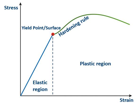
Figure 1: Stress Strain graph of a ductile material under uniaxial loading
In plasticity theory, materials exhibit different behaviors depending on whether their plastic response is influenced by strain rate, which is affected by the rate of loading. This leads to two main categories: rate-independent plasticity, where the material’s plastic behavior remains unchanged regardless of loading speed, and rate-dependent plasticity, where yield stress increases with faster loading due to strain rate effects.
This strain rate effect refers to how a material’s response changes with deformation speed, making materials stronger as strain rate increases. It is particularly important in applications involving dynamic or high-speed loading, such as impact, crash, explosion, and metal forming processes. The present discussion would be limited to rate independent material models.
The constitutive models for elastic-plastic behavior start with a decomposition of the total strain into elastic and plastic parts \(\in=\in^{el}+\in^{pl}\)
The stress is proportional to the elastic strain \(\in^{el}\) , i.e., \(\sigma=D\in^{el}\) and the evolution of plastic strain \(\in^{pl}\) is a result of the plasticity model.
1. Yield Criterion – Defines when a material transitions from elastic to plastic behavior. i.e., defines the point where the material stops behaving elastically and starts deforming plastically.
$$f(\sigma,\sigma_y)=0$$
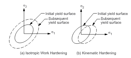
Figure 2: Types of Hardening Rules
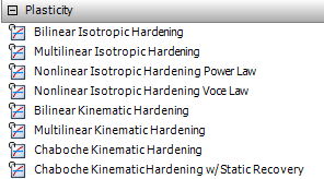
These models assume that the yield surface expands uniformly in all directions as the material hardens. They are suitable for monotonic loading conditions.
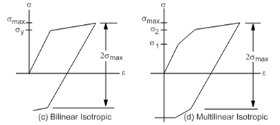
Uses a constant plastic modulus after yielding.
|
Constant
|
Meaning
|
Property
|
|---|---|---|
|
C1
|
\(\sigma_0\)
|
Yield stress
|
|
C2
|
\(E_p\)
|
Plastic tangent modulus
|
The multilinear hardening behavior is described by a piece-wise linear stress-total strain curve, starting at the origin and defined by sets of positive stress and strain values, as shown in this figure:
|
Constant
|
Meaning
|
Property
|
|---|---|---|
|
X
|
\({\varepsilon_i^{pl}}_{}\)
|
Plastic strain value
|
|
Y
|
\(\sigma_i\)
|
Stress Value
|
Captures more complex hardening behavior using empirical laws.
Power Law Hardening follows a power-law relationship between stress and plastic strain. The following table lists the required constants:
|
Constant
|
Meaning
|
Property
|
|---|---|---|
|
C1
|
\(\sigma_0\)
|
Initial yield stress
|
|
C2
|
N
|
Exponent
|
Voce Law Hardening models material behavior where there is rapid initial hardening after yielding, followed by a gradual saturation to a constant stress level. The following table lists the required constants:
|
Constant
|
Meaning
|
Property
|
|---|---|---|
|
C1
|
\(\sigma_0\)
|
Initial yield stress
|
|
C2
|
\(R_0\)
|
Linear Coefficient
|
|
C3
|
\(R_\infty\)
|
Exponential coefficient
|
|
C4
|
b
|
Exponential saturation parameter
|
|
Constant
|
Meaning
|
Property
|
|---|---|---|
|
C1
|
\(\sigma_0\)
|
Initial yield stress
|
|
C2
|
\(E_p\)
|
Plastic tangent modulus
|
|
Constant
|
Meaning
|
Property
|
|---|---|---|
|
P1
|
\(\varepsilon_i\)
|
Strain value
|
|
P2
|
\(\sigma_i\)
|
Stress value
|
Chaboche Kinematic Hardening w / Static Recovery: Static recovery (also known as thermal recovery) is a feature in kinematic hardening where the backstress (the shift of the yield surface) relaxes over time even when the material is unloaded or under small loads. It represents dislocation rearrangement and reduction of internal stresses during rest periods.
Static recovery is essential for modeling long-term cyclic loading, low-cycle fatigue, and creep-fatigue interactions.
|
Loading Type
|
Material Response
|
Recommended Hardening Model
|
Application
|
|---|---|---|---|
|
Single Loading (Monotonic)
|
No unloading/reloading expected
|
Isotropic Hardening (Bilinear, Multilinear, Nonlinear)
|
Static loading,
metal forming,
crash analysis
|
|
Simple Cyclic Loading (Loading → Unloading → Reloading)
|
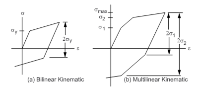
Yield surface shifts back and forth (Bauschinger Effect)
|
Kinematic Hardening (Bilinear Kinematic, Multilinear Kinematic)
|
Low-cycle fatigue,
repeated loading structures
|
|
Complex Cyclic Loading + Memory Effects
|
History-dependent behavior, mean stress relaxation
|
Combined Hardening (Chaboche Model)
|
Fatigue life prediction, creep-fatigue interaction in turbine blades, high-cycle fatigue of automotive components
|